In this post we explore the connections between standard Machine Learning methods and Bayesian inference. We also show how to build a Bayesian neural network without relying on specialized packages.
The first section is a refresher on Bayesian stats, then we discuss the Bayesian interpretation of your usual Machine Learning models, last we implement a Bayesian neural network in Jax.
Back to Bayesics
A common view of Machine Learning is as an optimization problem over a neural network’s parameters to minimize a loss function.
For example given a NN with parameters \(\theta\) we may aim to find
We recognize this as minimizing the mean squared error loss. Taking a probabilist view we recognize it from least squares regression, where we are finding \(\theta\) satisfying (assuming Gaussian errors). \[\hat{\theta} = \arg\max_{\theta} \log{p(x | \theta )}\]
In plain text this reads “which choice of \(\theta\) would make seeing this data the most likely?” Note, this does not answer the question “which \(\theta\) is the most likely given the data we’ve observed?”
Generally we are interested in estimating \(\theta\) based on the data \(p(\theta | x)\), not the other way around. The way forward is Bayes’ theorem:
The denominator \(p(x)\) is problematic, how are we supposed to figure out the objective likelihood of the data in the real world? \(p(x)\) forms a normalizing constant (w.r.t \(\theta\)) ensuring \(p( \theta | x)\) integrates to 1.
Bayes’ theorem is often reformulated as
\[p(\theta|x) \propto p(x|\theta)p(\theta)\]
where the right hand side is an unnormalized probability.
We have one other issue, what is \(p(\theta)\)? If we knew the parameters we wouldn’t be solving for them. Maybe we do have some hunch about the scale and behaviour of the parameters, so what if we assign \(\theta\) a probability distribution a priori? This distribution is a design choice we have to make and \(p(\theta\)) is called the prior distribution of \(\theta\), prior as in prior beliefs or assumptions.
Note that the improper prior \(p(\theta)=1\) would make \(p(\theta|x) \propto p(x|\theta)\) everywhere (and thus equal?).
Let’s start by implementing our own Bayesian linear regression. In the following sections we’ll work with log probabilities
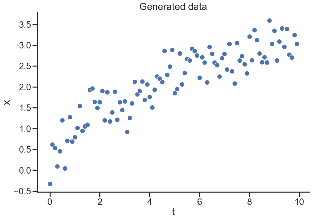
Let’s generate some data \(x = \sqrt{t} + \epsilon\).
import numpy as npnp.random.seed(123)import matplotlib.pyplot as pltimport seaborn as snssns.set_theme()sns.set_style("ticks")sns.color_palette("dark")plt.rc("axes.spines", top=False, right=False)plt.rc("figure", figsize= (12,8))# generate synthetic datat = np.arange(0,10, 0.1)x = t**0.5+ np.random.randn(len(t))*0.3sns.scatterplot(x=t, y=x);plt.title("Generated data");plt.xlabel("t");plt.ylabel("x");
Our model will be very simple, a linear model in 1 parameter without intercept.
We’ll use a \(N(0,1)\) prior on the regression parameter \(\theta\), encoding an assumption that it is relatively small. It’s a weakly informative prior that doesn’t nudge the model in any particular direction. For example if we suspect \(\theta>0\) we could have let the choice of prior reflect this prior belief.
We will also assume the likelihood \(p(x(t)| \theta) \sim N(\theta t,1)\) according to our linear model.
Next we want to define the log probabilities of \(p(x | \theta)\) and \(p(\theta)\): our likelihood and prior respectively.
def lm(theta, t):# our linear modelreturn theta*tdef logprob_norm(data, mu=0, sigma=1):# log of the normal pdfreturn-np.log(sigma) - np.log(2*np.pi)/2- (data - mu)**2/ (2* sigma**2)def logprob_prior(theta, mu=0, sigma=1):return logprob_norm(theta, mu, sigma)def logprob_likelihood(x, theta, t, sigma=1):return logprob_norm(x, lm(theta, t), sigma)
Now how do we sample from the posterior \(p(\theta | x)\) given these unnormalized log probabilities? There are many sophisticated ways to do this including HMC and SVI, but here we’ll use the Gumbel max trick.
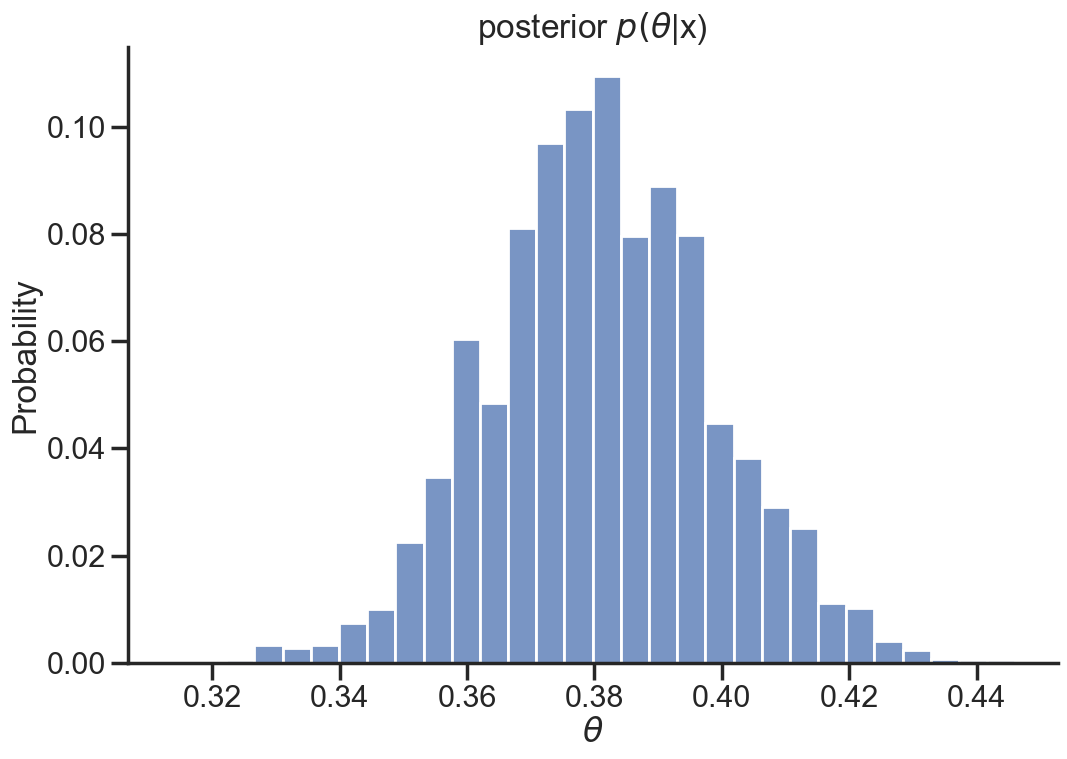
N_samples=10000log_posteriors = []thetas = []# for loop for relative readabilityfor _ inrange(N_samples):# sample from theta prior theta_prior = np.random.normal() thetas.append(theta_prior)# log probabilities of prior and likelihood lpp = logprob_prior(theta_prior) lpl = np.sum(logprob_likelihood(x, theta_prior, t))# log probability of posterior. lppost = lpp + lpl log_posteriors.append(lppost)log_posteriors=np.array(log_posteriors)posterior_samples=[]for _ inrange(N_samples):# use standard gumbel variables to sample from theta based on the log probs gumbels=np.random.gumbel(0,1,N_samples) theta_ind=np.argmax(log_posteriors + gumbels) posterior_samples.append(thetas[theta_ind])
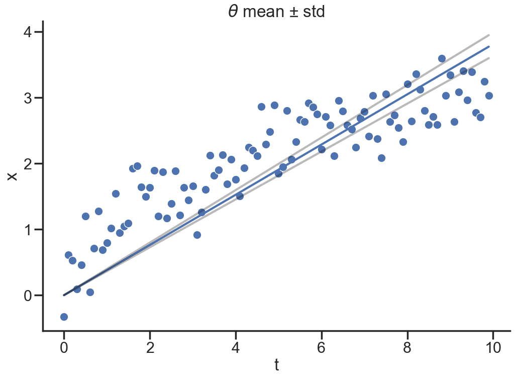
We have successfully sampled from the posterior distribution \(p(\theta|x)\) and found that \(\theta \approx 0.38\) with quite some certainty.
What about the predicted values \(\tilde{x}(t)\) given this model? This is also probabilistic given the posterior distribution of \(\theta\). These values are distributed according to the posterior predictive distribution \[p(\tilde{x}(t)|x) = \int p(\tilde{x}(t)|\theta ) p(\theta|x(t)) d\theta\]
This involves sampling \(\tilde{x}(t) \sim N(\mu_x = \theta t, \sigma_x = 1)\), but in the following sections we’ll drop the aleatoric uncertainty \(\sigma_x\) and only consider the epistemic uncertainty in the model parameters.
We’re essentially looking for the probability of the mean of \(\tilde{x}\) given all our data x by sampling \(\theta\) from the posterior.
For example \(\tilde{x}(t=4).\)
posterior_predictive_samples=[lm(theta, 4) for theta in posterior_samples]sns.histplot(posterior_predictive_samples, bins=30, stat="probability");plt.title(r"$\mathbf{E}[\tilde{x}(t=4)|\theta]$");plt.xlabel(r"$\tilde{x}(t=4)$");
The square root of 4 is actually 2, maybe it’s time to improve the model?
Machine Learning Problem
Let’s explore the NN mentioned in the beginning, we define a model in Flax NNX and minimize the MSE.
import jaximport jax.numpy as jnpfrom flax import nnxfrom jax.random import PRNGKeyimport optaximport pandas as pd
class NN(nnx.Module):def__init__(self, dim_in=1, dim_out=1, n_hidden =3, act = nnx.sigmoid, *, key):self.act = act keys = jax.random.split(key, 3)self.layer1 = nnx.Linear(dim_in, n_hidden, rngs = nnx.Rngs(params=keys[0]))self.layer2 = nnx.Linear(n_hidden, n_hidden, rngs = nnx.Rngs(params=keys[1]))self.layer3 = nnx.Linear(n_hidden, dim_out, rngs = nnx.Rngs(params=keys[2]), use_bias=False)def__call__(self, x): x =self.layer1(x) x =self.act(x) x =self.layer2(x) x =self.act(x)returnself.layer3(x)defapply(self, params, x):# will be used later nnx.update(self, params)returnself.__call__(x)@nnx.jitdef loss_fn(model, t, x): y = model(t)return jnp.mean((x-y)**2)
Overfitting aside we have found parameters \(\theta\) of the neural network \(f_{\theta}\) that minimize our loss function:
\[\Vert x - f_{\theta}(t) \Vert^2\]
Remember we generated the data with normal i.i.d noise, in a probabilistic setting it would be suitable to model the data generating distribution as
\[ x(t) \sim N(f_{\theta}(t), \sigma)\]
Performing a maximum likelihood fit we would maximize the log likelihood \[\log {p(x(t) | \theta)} = \log{ \frac{e^{-\frac{\Vert x-f_{\theta}(t) \Vert^2}{2 \sigma^2}}}{\sqrt{2\pi \sigma^2}}} \propto C - \Vert x - f_{\theta}(t) \Vert^2\]
Maximizing the Gaussian log likelihood is the same as minimizing our MSE loss function.
One possible remedy for overfitting is regularization of the neural network parameters, for example \(L_2\)-regularization would add a term \(\beta \Vert \theta \Vert^2\) to the loss function, penalizing large model weights. This generally has a smoothing effect on the output.
The loss function would become \[\Vert x - f_{\theta}(t) \Vert^2 + \beta \Vert \theta - 0 \Vert^2\]
The connection to our Bayesian linear regression is obvious if we flip the sign, these are the unnormalized negative log probabilities of a Gaussian prior and likelihood. Adding regularization to our loss function turns the (frequentist) maximum likelihood estimate into a (Bayesian) maximum a posteriori estimate (MAP).
If you were using \(L_2\)-regularization you were a Bayesian all along! Whether you call it regularization, shrinkage or a prior the effect is the same: constraining parameter values. Similarly, when you use MSE loss you’re solving the same mathematical problem as Gaussian maximum likelihood, i.e. under the hood you are assuming Gaussian i.i.d errors. Probability theory just refuses to go away!
\(L_1\)-regularization? A Laplace prior.
MAE loss? Laplace likelihood.
Bayesian Neural Network
We learned that the standard neural network has a Bayesian interpretation, but something is missing. We didn’t manage to sample from our posterior \(p(\theta | x)\), we just found a point estimate of \(\theta\). In order to be fully Bayesian we’d like to average over this posterior distribution when predicting new values.
Drawing samples from the posterior is a difficult problem in general, the standard way is to sample using MCMC (typically HMC) or SVI. These samplers can be found in a variety of packages and part of excellent PPLs like Numpyro, PYMC and Turing.jl. Here we will try out a NUTS sampler from the Blackjax package.
We’ll use the arbitrary priors \(p(\theta_i) \sim N(0,100)\) on the neural network parameters. This is a very uninformative prior that will most likely cause numerical instability for more complex models and data. The prior log likelihood is proportional to \(1/\sigma^2\), in this case roughly equivalent to a \(L_2\)-regularization parameter \(\beta \approx\) 1e-4.
@jax.jitdef logprior_fn(params): leaves, _ = jax.tree_util.tree_flatten(params) flat_params = jnp.concatenate([jnp.ravel(a) for a in leaves])return jnp.sum(logprob_norm_jax(flat_params, 0, 100))@jax.jitdef loglikelihood_fn(params, data): t, x = datareturn jnp.sum(logprob_norm_jax(x, model.apply(params, t), .5 ))@jax.jitdef logdensity_fn(params):return logprior_fn(params) + loglikelihood_fn(params, data)
model = NN(act=nnx.sigmoid ,key=rng_key)state = nnx.state(model)param = state.filter(nnx.Param)
adapt = blackjax.window_adaptation( blackjax.nuts, logdensity_fn, target_acceptance_rate=0.8)rng_key, warmup_key = jax.random.split(rng_key)# warm up the model in order to reach equilibrium(last_state, parameters), _ = adapt.run(warmup_key, param, num_warmup)kernel = blackjax.nuts(logdensity_fn, **parameters).step
# apply model with weights sampled from the posterior distribution, e.g. draw x from the posterior predictiveres = jax.vmap(eval_fn, in_axes=(0, None))(posterior_params, t).squeeze()# predict out of samplet_oos=jnp.arange(0,20,.1)res_oos = jax.vmap(eval_fn, in_axes=(0, None))(posterior_params, t_oos).squeeze()
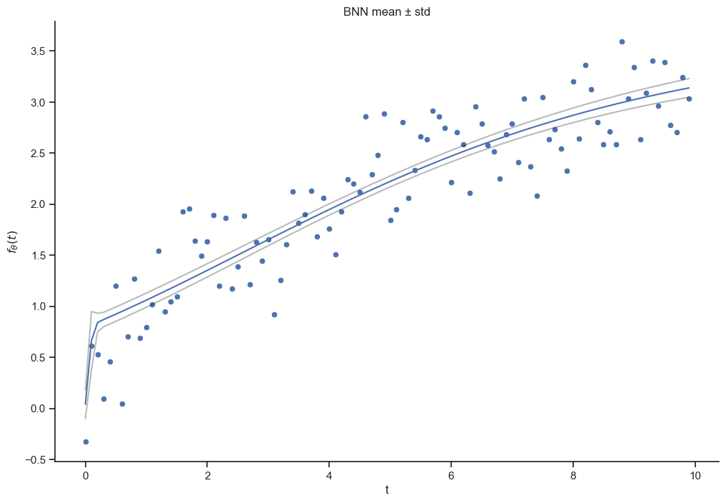
Here we’ve taken posterior samples of the neural network parameters \(\theta\) and evaluated the model with them, collecting the different outputs. This yields samples of the model’s mean prediction given \(\theta\) from the posterior.
It is also possible to sample from the full posterior predictive distribution by including the aleatoric uncertainty from the likelihood \(\sigma\), but we’ll stick with the mean prediction. You can also estimate \(\sigma\), here we arbitrarily set it to \(\sigma=0.5\). If this is your goal I would recommend using a PPL.
means=df_res.mean(axis=1)stds = df_res.std(axis=1)sns.scatterplot(x = t, y = x);sns.lineplot(x = t, y = means)sns.lineplot(x = t, y = means + stds, color="k", alpha=0.3);sns.lineplot(x = t, y = means - stds, color="k", alpha=0.3);plt.title(r"BNN mean ± std");plt.xlabel("t");plt.ylabel(r"$f_{\theta}(t)$");
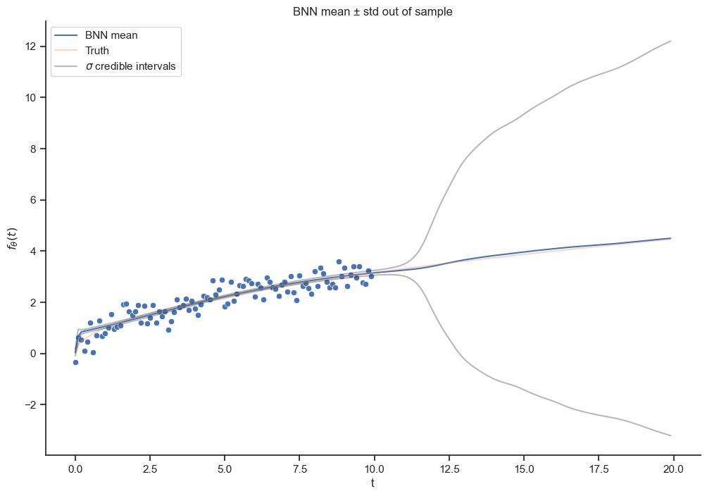
means=df_oos.mean(axis=1)stds = df_oos.std(axis=1)sns.lineplot(x=t_oos, y=means);sns.lineplot(x=t_oos, y=np.sqrt(t_oos), alpha=0.3)sns.lineplot(x=t_oos, y=means + stds, color="k", alpha=0.3);sns.lineplot(x=t_oos, y=means - stds, color="k", alpha=0.3);sns.scatterplot(x=t, y=x);plt.title(r"BNN mean ± std out of sample");plt.xlabel("t");plt.ylabel(r"$f_{\theta}(t)$");plt.legend(["BNN mean", "Truth", r"$\sigma$ credible intervals"]);
When using a BNN our predictions are generally samples drawn from the posterior predictive distribution, this has the benefit of informing us about the model’s uncertainty (about the model parameters in this case). In-sample the model fits the data quite well with no obvious overfitting. We see that the standard deviation grows when we try to extrapolate. Maybe someday LLMs will have this feature instead of confidently recommending eating rocks.